Faster correlation mining in Python

Introduction

Calculating and identifying correlations between variables is a key component of the modern data science workflow. For me, it is especially relevant because of the importance biomarker discovery plays in cancer genomics. In this post, I explain key methods used in correlation mining, provide examples of their usage, and describe tricks that can be used to speed up computation in practice.

The problem

A common practice in modern genomics, and hypothesis-free science in general, is to mine relationships by computing correlations between a variable of interest and many other variables. For instance, to find genes that may predict the response of cancers to a drug, one might correlate sensitivity values of the drug among cell lines to expression levels of every single gene, with the hope that some genes might be indicative of response to the drug.

The results of such analyses are often described through volcano plots, where one plots the effect size (a variable indicating the strength of association, such as a Pearson or Spearman correlation) on the x-axis versus the significance, or P value of such correlations on the y-axis. For instance, in the following figure, the authors show that WRN, a gene that encodes a DNA-maintaining protein, could be a potential drug target in microsatellite-instability (MSI) cancers. This is shown by the fact that WRN dependency values among cell lines (i.e. how sensitive cell lines are to depletion of WRN) are especially strongly associated with MSI status compared to every other profiled gene.

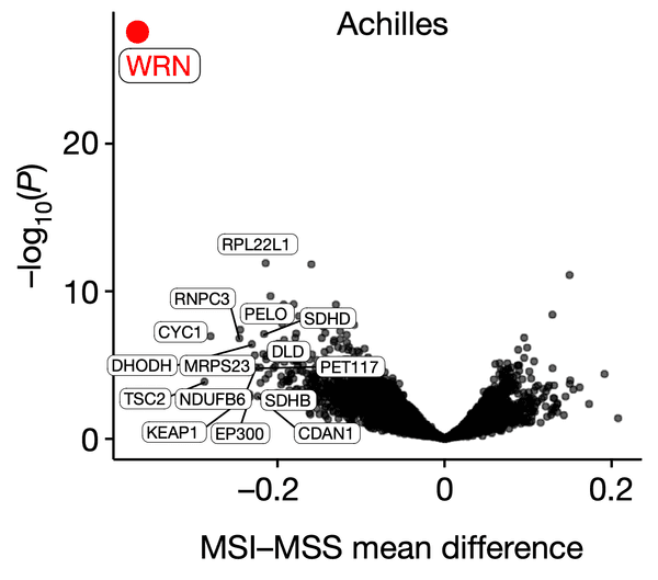
WRN dependency is strongly associated with the MSI phenotype. Source: WRN helicase is a synthetic lethal target in microsatellite unstable cancers.

Beyond finding biomarkers that might predict the expression of a single gene or resistance to a single drug, we are also frequently interested in computing "all vs all" associations, for instance between all genes and all drugs to find new and strong associations in general. In systems biology, for instance, we often compute correlation networks within datasets such as gene expression to find modules of genes with related or coordinated functions. The computation of these large matrices can be quite expensive – for instance, with around 20,000 genes in the genome, we have $\frac{(20000)(20000-1)}{2}\approx2\times10^8$ distinct pairs to compare, which is a nontrivial task. There are several ways to approach this challenge, and the differences in speed are large enough to justify a closer look.

The solution(s)

The fastest solution to implement pairwise correlation calculation is to write a for loop, where we go through every pair of variables in dataset $X$ and compare them with every pair of variables in dataset $Y$:

for variable x in X:
  for variable y in Y:
    compute effect_size(x,y)
    compute p_value(x,y)

Although this is a fast solution to write, it is ultimately quite slow when implemented in high-level languages like Python or R (see this thread for an in-depth explanation). I ended up using variations of this scheme for a couple of weeks before it quickly became apparent that a faster and more organized approach was required.

To explain the methods used, I will first stratify them by the kinds of variables we are comparing. In particular, our variable may be continuous, like a measure of a gene's expression level or dependency, or it may be categorical, such as the presence of a mutation or the tissue type of a cell line. As a result, we can consider three combinations of compared variables: continuous vs. continuous, continuous vs. categorical, and categorical vs. categorical. For each combination, we would like an effect size statistic quantifying the strength of an association as well as a statistical test for calculating the significance of this effect size.

Continuous vs. continuous

Our first type of comparison is between two continuous variables. The most widely-used measure of association in this context is the Pearson correlation coefficient, which is often denoted as $r$. The formal definition of the correlation coefficient is the covariance between two variables divided by the product of their standard deviations, and therefore may be seen as a normalized covariance.

In other words, given two paired samples $x$ and $y$, we can compute the correlation coefficient $r_{x,y}$ as

where $\text{cov}(x,y)$ is the covariance and $s_x,s_y$ are the respective standard deviations.

If we let $n$ be the number of samples in each variable, then this can be expanded to

where $\bar{x},\bar{y}$ are the respective means. Intuitively, the Pearson correlation expresses how well two variables may be related to each other via a linear function (formally, the square of the correlation is equivalent to the fraction of the variance in $y$ that may be attributed to $x$ through a linear relationship.)

A close relative of the Pearson correlation coefficient is the Spearman rank correlation coefficient, which is denoted as $\rho$, or rho. The Spearman correlation between two variables is equivalent to the Pearson correlation between their ranks, where rank refers to the numerical place of an object in the sample. For instance, a sample $(0.5,0.2,0.8)$ has the respective ranks $(2,1,3)$ in ascending order. Because the Spearman correlation measures how well ranks are linearly related to each other, it reflects how well two variables may be related by any monotonic function. This is particularly useful for data mining in biology because many relationships are nonlinear; for instance, the effect of one gene's expression in regulating that of another may instead have an exponential relationship.

Now, having defined the statistics of interest, we can consider how they might be optimized computationally. In particular, to make our code faster while sticking to Python, we can revisit the way such associations are calculated and try to rewrite them in a vectorized format.

Recalling our earlier definition of the Pearson correlation coefficient, we see that if we let $\vec{x},\vec{y}$ be vectors of samples $x,y$, then this is equivalent to

Here we assume that operations like $\vec{x}-\bar{x}$ have the scalar broadcasted to a constant vector. If we represent our datasets as matrices where each column vector is a sample, then our vector-pair formula generalizes well given the connection between matrix multiplication and vector dot products – recall that for two matrices $A\in \mathbb{R}^{l\times m}, B\in\mathbb{R}^{m\times n}$, the entry $[AB]_{i,j}$ is equivalent to the dot product of the $i$-th column of $A$ and the $j$-th row of $B$.

In particular, suppose $A$ and $B$ are our dataset matrices of $m, n$ respective variables and $k$ samples. In other words, let

where $\vec{y}_i,\vec{x}_i$ are the respective column vectors of $A,B$. Taking our vectorized Pearson correlation method, we can reformulate this as follows, where a_mat and b_mat are our matrix objects:

residuals_a = a_mat - a_mat.column_means
residuals_b = b_mat - b_mat.column_means

a_residual_sums = residuals_a.column_sums
b_residual_sums = residuals_b.column_sums

residual_products = dot_product(residuals_a.transpose, residuals_b)

sum_products = sqrt(dot_product(a_residual_sums, b_residual_sums))

correlations = residual_products / sum_products

When implemented with NumPy, this allows us to take advantage of faster underlying implementations. As a result, computing Pearson correlations between matrices becomes nearly 100x faster. With Spearman correlations, we get an additional speed boost because we can use vectorized ranking methods as well, resulting in a nearly 200x speed boost over the standard SciPy implementation.

Having considered the case where both our variables are continuous, we now turn to situations where one of our variables is discontinuous, or categorical.

Continuous vs. categorical

In the simplest case, suppose we want to compare a binary variable against a continuous one, which can be seen as comparing two groups of the continuous one: positive versus negative.

One measure of difference might be to compute the difference in the means or medians of the two groups; however, this method does not provide a comparable measure of effect size between multiple variables which may have different scales. To get a normalized sense of correlation, we can employ the rank-biserial correlation. Just like the Pearson and Spearman correlations, the rank-biserial correlation also varies from $-1$ to $1$, with a value of $-1$ indicating a perfect negative relationship, a value of $0$ indicating no relationship, and a value of $1$ indicating a perfect positive relationship.

First, let us label our two groups as either positive ($+$) and a negative ($-$) with respective sample sizes $n_+,n_-$. Now, define two intermediate variables $R_+,R_-$ as the sums of the ranks in each group, where the rank is assigned based on the merged groups. Using these rank sums, we compute another intermediate statistic $U_+$ as follows:

Let's consider what this formula tells us.

• Consider the extreme case in which all the samples in the positive group are lower than those in the negative group. In this scenario, the ranks of these positive samples would be $\{0,\dots,n_+\}$, and their sum $R_+$ would be $\frac{n_+(n_++1)}{2}$. Therefore, we see that $U_+$ is $0$ when the positive group is completely below the negative one.
• On the other end, consider the extreme case where all samples in the positive group are higher than those of the negative group. In this scenario, the ranks of these positive samples would be $\{n_-+1,\dots,n_-+n_+\}$, and their sum $R_+$ would be $\frac{n_+(n_++1)}{2}+n_+n_-$. In this case, we see that $U_+=n_+n_-$ when the positive group is completely above the negative one.

Therefore, we see that $U_+$ ranges from $0$ to $n_-n_+$. To normalize this statistic to the range $[-1,1]$, we can multiply it by $\frac{2}{n_+n_-}$ and subtract one, which leads us to the formula for the rank-biserial correlation:

Note that another way to derive this is from the definition of the rank-biserial as the difference between the fraction of favorable pairs $f$ minus the fraction of unfavorable pairs $u$. The number of favorable pairs $f$ is indicated by $U_+$, so we see again that

Along with $U_+$, we also have a $U_-$ statistic computed from the rank sum and sample size of the negative group as one would expect: $U_-=R_--\frac{n_-(n_-+1)}{2}$. It follows by some simple algebra that $U_++U_-=n_1n_2$.

By taking the minimum of $U_+,U_-$, we have the $U$ statistic, which forms the basis of the Mann-Whitney $U$ test for calculating the significance of this association between a continuous and a binary variable. Because the calculation of a significance value for the test is often computationally infeasible for large sample sizes, a normal approximation for $U$ is often used. Note that the Mann-Whitney $U$ test requires a few assumptions that may be tricky to meet in practice:

• The observations are all independent of one another.
• Under the null hypothesis, the distributions of continuous variable in the positive and negative groups are equivalent.
• The sample size is large enough (above 20 in each group) for $U$ to be approximately normally-distributed under the null hypothesis.

There is also the edge case of correcting for possible ties in the continuous variable. This is explained on the Wikipedia page and can be handled using scipy.stats.tiecorrect, which is used by the SciPy Mann-Whitney $U$ implementation.

Having defined the calculation of the rank-biserial correlation as well as the $U$ statistic, we can consider how a vectorized implementation would work. A similar formulation of the vectorized method can be used for the calculation of the Mann-Whitney $U$ test for comparing binary and continuous samples.

Recall that with the Mann-Whitney $U$ test, there are two particular quantities of interest: $U_+=R_+-\frac{n_+(n_+ + 1)}{2}$, with $R_+$ being the sum of the ranks in the positive sample group, and $r=\frac{2U_+}{n_+n_-}-1$. To vectorize these, we can begin by first applying the axis-level ranking methods previously used for computing Spearman correlations, after which we create positive and negative binary indicator matrices to enable the rank sum calculations as dot products. In particular:

a_ranks = a_mat.apply(ranks_within_columns)

b_pos = b_mat.astype(float)
b_neg = b_mat.astype(float)

pos_counts = b_pos.sum(axis=0)
neg_counts = b_neg.sum(axis=0)

pos_counts = repeat(pos_counts, num_a_cols)
neg_counts = repeat(neg_counts, num_a_cols)

Now, we can calculate $U_+$ and $U_-$ as follows.

pos_ranks = dot_product(a_ranks.transpose, b_pos)

u*pos = pos_ns * neg*ns + (pos_ns * (pos_ns + 1)) / 2.0 - pos_ranks
u_neg = pos_ns * neg_ns - u_pos

Note the use of the * operator to denote elementwise matrix multiplication, or the Hadamard product.

Next, we calculate the rank-biserial correlation coefficient using our formula from above:

n_prod = pos_ns * neg_ns
zero_prod = n_prod == 0
n_prod[zero_prod] = 1

rank*biserial = 2 * u*pos / (pos_ns * neg_ns) - 1

effects[zero_prod] = 0

For categorical variables with more than two categories, we use other statistical tests, such as the ANOVA and the Kruskall-Wallis H test. These are more difficult to translate into vectorized formats, and the Mann-Whitney U test is usually enough for most categorical applications.

Categorical vs. categorical

Having analyzed two types of comparisons, we now consider the last: if both of our variables are categorical. In the simplest case, we can consider a scenario where we want to compare two binary traits. In this case, we can employ a measure called the odds ratio, which measures the difference in odds between a pair of conditions. The odds ratio is $1$ when the odds are the same in each condition, with values below or above $1$ indicating a difference in odds. Note that as a ratio between ratios, the odds ratio must be positive.

Here, we will explore a vectorized method to calculate the odds ratios and P-values when comparing two sets of binary variables. Suppose we have two binary samples $x,y$ each of $n$ elements. Consider the respective binary sample vectors $\vec{x},\vec{y}$ represented by each element being $0$ or $1$. To calculate the odds ratio, we need to compute a contingency table that is equivalent to

Here, the notation $x'$ means the binary opposite of $x$, such that $\vec{x}'=1-\vec{x}$. Since the $\text{AND}$ operation is just adding up the values of the two vectors that are both $1$, it is equivalent to the dot product operation between vectors, which we can expand to the dot product between the two matrices where the sample vectors are represented as columns. The odds ratio is then equivalent to

Therefore, our code for performing the contingency matrix calculation might look something like this:

A_pos = a_mat
A_neg = 1 - a_mat
B_pos = b_mat
B_neg = 1 - b_mat

AB = dot_product(A_pos.transpose, B_pos)
Ab = dot_product(A_pos.transpose, B_neg)
aB = dot_product(A_neg.transpose, B_pos)
ab = dot_product(A_neg.transpose, B_neg)

Having computed the contingency table cells, we can use elementwise multiplication and division to compute the odds ratios. We also handle cases where the denominator may be zero. In particular, we do:

numer = AB _ ab
denom = aB _ Ab

zero_denom = denom == 0
denom[zero_denom] = 1

oddsrs = numer / denom
oddsrs[zero_denom] = -1

Next, we can stack the four matrices into a single tensor of shape $(4, \text{num\textunderscore a\textunderscore columns}, \text{num\textunderscore b\textunderscore columns})$, upon which we can apply numpy.apply_along_axis to compute the significance values from Fisher's exact test.

The speed of Fisher's exact test can further be boosted by a factor of nearly 50 by using a faster implementation provided by painyeph. The use of vectorized matrix multiplication itself lends a roughly 4-8x speed boost. Therefore, the combination of vectorized methods and an alternative significance calculation algorithm results in an overall 200x reduction in running time compared to a loop implementing the standard SciPy method.

Comparing categorical variables when more than two categories is involved is a bit trickier: if we have enough counts in each category combination, we can use the $\chi^2$ test. Otherwise, if our contingency tables are small enough, extensions to Fisher's exact test on $2\times 2$ tables can be used. Note that if we do not have enough counts to use a $\chi^2$ test (which depends on sufficient counts to assume the test statistic is $\chi^2$-distributed under the null distribution), we can also use permutation/randomization testing to get an accurate estimate of significance.

More faster

Speeding up our calculations by vectorizing them in NumPy is by no means the end of the road. We can optimize further using a couple of well-known tricks: using alternative NumPy backends, just-in-time compilation, and GPU acceleration.

The NumPy backend for most machines is often built from BLAS and LAPACK, which are fairly decent packages. However, for certain scenarios, backends such as ATLAS, MKL, and OpenBLAS may be faster. Online benchmarks suggest that matrix multiplication may be up to 20x faster using these other implementations. Right now, my default implementation used in benchmarking is OpenBLAS, though switching to MKL may yield further speed boosts in the future.

Just-in-time (JIT) compilers for Python allow us to optimize certain functions by compiling them to machine code right before execution. This is implemented by packages such as Numba, which supports a wide range of Python and NumPy functions. An additional feature of Numba is the fact that it can parallelize operations, which allows us to make more use of the multiple cores at our disposal. I have yet to implement Numba yet in my workflow, but preliminary results suggest that it should yield a sizable speed boost.

GPU acceleration allows us to make use of the highly-parallel architectures of graphics chips to provide additional speed boosts. However, this is a less universal solution because we must have a GPU to start with as well as the proper device drivers. So far, I have only managed to implement NVIDIA-specific GPU acceleration on Mann-Whitney $U$ tests. I was able to accomplish this because the required probability distribution function (in particular, the survival function for the normal distribution) is also implemented in cupy, the acceleration library used. Unfortunately, the I'm still looking for the required statistical methods for Pearson regression (the Student's t distribution) and Fisher's exact test (the natural logarithm of the absolute value of the Gamma function).

The package

As I encountered more and more situations where these methods were to be applied, I gradually organized my code into a package – many. This package provides both the naive and vectorized implementations for all cases discussed above, test cases for validating the accuracy of the vectorized methods, and thorough benchmarks verifying the performance improvements.